[1]:
from mimic.utilities import *
from mimic.utilities.utilities import plot_CRM, plot_CRM_with_intervals

from mimic.model_infer.infer_CRM_bayes import *
from mimic.model_infer import *
from mimic.model_simulate import *
from mimic.model_simulate.sim_CRM import *

import numpy as np
import pandas as pd
import seaborn as sns
import matplotlib.pyplot as plt

import arviz as azS
import pymc as pm
import pytensor.tensor as at
import pickle
import cloudpickle

from scipy import stats
from scipy.integrate import odeint
WARNING (pytensor.tensor.blas): Using NumPy C-API based implementation for BLAS functions.
Bayesian inference to infer the parameters of a Consumer Resource model
The Consumer Resource equation based on the MacArthur model takes the form
where:
\(N\) is the concentration of each species
\(\tau\) is the species timescale
\(m\) is the species mortality rate
\(R\) is the concentration of each resource
\(r\) is the resource timescale
\(w\) is the quality of each resource
\(K\) is the resource capacity
\(c\) is each species’ preference for each resource
Unlike the gLV, the CRM is not linearised, so the DifferentialEquation function from pymc is utilised to solve the ODEs within the inference function. This can take a while if inferring all parameters, so below we demonstrate run_inference by inferring only one parameter (c) while the rest remain fixed, where inferring all parameters takes longer.
Read in simulated data
The data was simulated examples-sim-CRM.ipynb
[ ]:
with open("params-s2-r2.pkl", "rb") as f:
    params = pickle.load(f)
tau = params["tau"]
w = params["w"]
c = params["c"]
m = params["m"]
r = params["r"]
K = params["K"]


# read in the data

data = pd.read_csv("data-s2-r2.csv")

times = data.iloc[:, 0].values
yobs = data.iloc[:, 1:6].values

print(params)
{'num_species': 2, 'num_resources': 2, 'tau': array([0.6, 0.9]), 'w': array([0.5, 0.6]), 'c': array([[0.25, 0.08],
       [0.06, 0.22]]), 'm': array([0.25, 0.28]), 'r': array([0.4 , 0.35]), 'K': array([5., 6.])}
Infer parameter c only
While parameters tau, m, r, w and K remain fixed to true values generated by the simulation. Any combination of parameters can be inferred by providing the prior_mean and prior_sigma instead of the true value
[17]:
num_species = 2
num_resources = 2
# fixed parameters
tau = params["tau"]
#c = params["c"]
m = params["m"]
r = params["r"]
w = params["w"]
K = params["K"]
# Define prior for c (resource preference matrix)
prior_c_mean = [[0.2, 0.1],[0.1, 0.2]]
prior_c_sigma = [[0.1, 0.1],[0.1, 0.1]]
# Sampling conditions
draws = 50
tune = 50
chains = 4
cores = 4
inference = inferCRMbayes()
inference.set_parameters(times=times, yobs=yobs, num_species=num_species, num_resources=num_resources,
tau=tau, w=w, K=K, r=r, m=m,
prior_c_mean=prior_c_mean, prior_c_sigma=prior_c_sigma,
draws=draws, tune=tune, chains=chains, cores=cores)
idata = inference.run_inference()
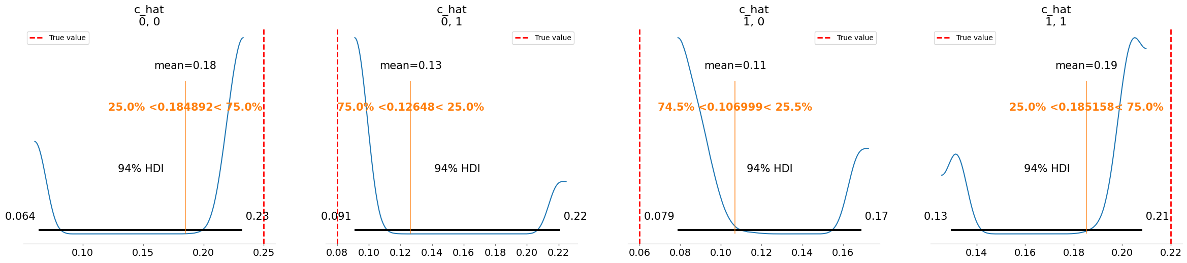
# To plot posterior distributions
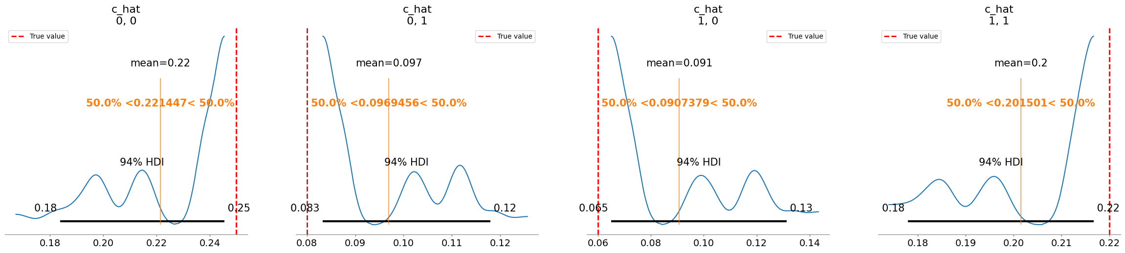
inference.plot_posterior(idata, true_params=params)
summary = az.summary(idata, var_names=["c_hat", "sigma"])
print(summary[["mean", "sd", "r_hat"]])
# Save posterior samples to file
az.to_netcdf(idata, 'model_posterior.nc')
times shape: (100,)
yobs shape: (100, 4)
Number of species: 2
Number of resources: 2
Only 50 samples per chain. Reliable r-hat and ESS diagnostics require longer chains for accurate estimate.
tau_hat is fixed
w_hat is fixed
c_hat is inferred
m_hat is fixed
r_hat is fixed
K_hat is fixed
=== RSME ===
RMSE: 1.904265
Data scale: 4.327
Model scale: 3.503
First few predictions: [[10.         10.         10.         10.        ]
 [13.36863656 11.58977536  6.35498361  4.80303315]
 [15.40186487 12.3577566   4.3663791   2.43231611]]
First few observations: [[ 9.99394166  9.89957073  9.96255863 10.02837974]
 [12.00265551 11.21044161  6.20330201  6.50836833]
 [13.3618914  12.04261137  4.18667318  4.59287508]]
nsp_tensor: [2], nr_tensor: [2]
tau_hat: [0.6 0.9], w_hat: [0.5 0.6]
c_hat: [[0.17186305 0.30983875]
 [0.09373503 0.29257562]], m_hat: [0.25 0.28]
r_hat: [0.4  0.35], K_hat: [5. 6.]
theta: [2.         2.         0.6        0.9        0.5        0.6
 0.17186305 0.30983875 0.09373503 0.29257562 0.25       0.28
 0.4        0.35       5.         6.        ]
Initial conditions (y0): [10. 10. 10. 10.]
Auto-assigning NUTS sampler...
Initializing NUTS using jitter+adapt_diag...
Multiprocess sampling (4 chains in 4 jobs)
NUTS: [sigma, c_hat_vals]
/home/cclare/projects/CRM/MIMIC/MIMIC_env/lib/python3.10/site-packages/pymc/ode/ode.py:131: ODEintWarning: Illegal input detected (internal error). Run with full_output = 1 to get quantitative information.
  sol = scipy.integrate.odeint(
/home/cclare/projects/CRM/MIMIC/MIMIC_env/lib/python3.10/site-packages/pymc/ode/ode.py:131: ODEintWarning: Excess accuracy requested (tolerances too small). Run with full_output = 1 to get quantitative information.
  sol = scipy.integrate.odeint(
 lsoda--  warning..internal t (=r1) and h (=r2) are       such that in the machine, t + h = t on the next step
       (h = step size). solver will continue anyway      in above,  r1 =  0.0000000000000D+00   r2 =  0.0000000000000D+00
 intdy--  t (=r1) illegal            in above message,  r1 =  0.1000000000000D+00
      t not in interval tcur - hu (= r1) to tcur (=r2)
      in above,  r1 =  0.0000000000000D+00   r2 =  0.0000000000000D+00
 intdy--  t (=r1) illegal            in above message,  r1 =  0.2000000000000D+00
      t not in interval tcur - hu (= r1) to tcur (=r2)
      in above,  r1 =  0.0000000000000D+00   r2 =  0.0000000000000D+00
 lsoda--  trouble from intdy. itask = i1, tout = r1      in above message,  i1 =         1
      in above message,  r1 =  0.2000000000000D+00
 lsoda--  at t (=r1), too much accuracy requested         for precision of machine..  see tolsf (=r2)       in above,  r1 =  0.1000000000000D+00   r2 =                  NaN
/home/cclare/projects/CRM/MIMIC/MIMIC_env/lib/python3.10/site-packages/pymc/ode/ode.py:131: ODEintWarning: Illegal input detected (internal error). Run with full_output = 1 to get quantitative information.
  sol = scipy.integrate.odeint(
/home/cclare/projects/CRM/MIMIC/MIMIC_env/lib/python3.10/site-packages/pymc/ode/ode.py:131: ODEintWarning: Excess work done on this call (perhaps wrong Dfun type). Run with full_output = 1 to get quantitative information.
  sol = scipy.integrate.odeint(
 lsoda--  warning..internal t (=r1) and h (=r2) are       such that in the machine, t + h = t on the next step
       (h = step size). solver will continue anyway      in above,  r1 =  0.0000000000000D+00   r2 =  0.0000000000000D+00
 intdy--  t (=r1) illegal            in above message,  r1 =  0.1000000000000D+00
      t not in interval tcur - hu (= r1) to tcur (=r2)
      in above,  r1 =  0.0000000000000D+00   r2 =  0.0000000000000D+00
 intdy--  t (=r1) illegal            in above message,  r1 =  0.2000000000000D+00
      t not in interval tcur - hu (= r1) to tcur (=r2)
      in above,  r1 =  0.0000000000000D+00   r2 =  0.0000000000000D+00
 lsoda--  trouble from intdy. itask = i1, tout = r1      in above message,  i1 =         1
      in above message,  r1 =  0.2000000000000D+00
/home/cclare/projects/CRM/MIMIC/MIMIC_env/lib/python3.10/site-packages/pymc/ode/ode.py:131: ODEintWarning: Excess accuracy requested (tolerances too small). Run with full_output = 1 to get quantitative information.
  sol = scipy.integrate.odeint(
lsoda-- at t (=r1), too much accuracy requested for precision of machine.. see tolsf (=r2) in above, r1 = 0.1000000000000D+00 r2 = NaN
Sampling 4 chains for 50 tune and 50 draw iterations (200 + 200 draws total) took 79 seconds.
There were 63 divergences after tuning. Increase `target_accept` or reparameterize.
The number of samples is too small to check convergence reliably.
Parameter tau_hat not found in posterior samples, skipping plot.
Parameter w_hat not found in posterior samples, skipping plot.
Plotting posterior for c_hat
Added true value line for c_hat: [[0.25 0.08]
 [0.06 0.22]]
Parameter m_hat not found in posterior samples, skipping plot.
Parameter r_hat not found in posterior samples, skipping plot.
Parameter K_hat not found in posterior samples, skipping plot.
              mean     sd  r_hat
c_hat[0, 0]  0.221  0.022   3.40
c_hat[0, 1]  0.097  0.013   3.40
c_hat[1, 0]  0.091  0.024   3.35
c_hat[1, 1]  0.202  0.014   3.14
sigma[0]     0.189  0.098   3.18
[17]:
'model_posterior.nc'
[18]:
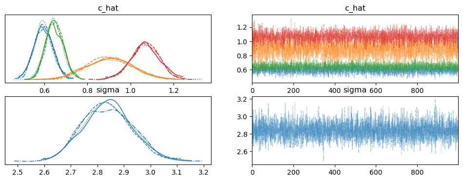
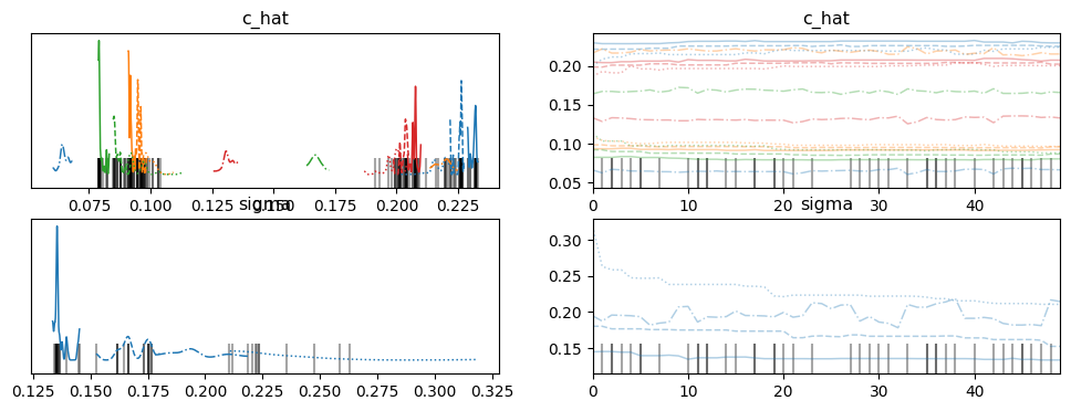
# Plot the trace of the posterior samples
az.plot_trace(idata, var_names=["c_hat", "sigma"])
[18]:
array([[<Axes: title={'center': 'c_hat'}>,
        <Axes: title={'center': 'c_hat'}>],
       [<Axes: title={'center': 'sigma'}>,
        <Axes: title={'center': 'sigma'}>]], dtype=object)
[19]:
# Plot the CRM
init_species = 10 * np.ones(num_species+num_resources)
# inferred parameters
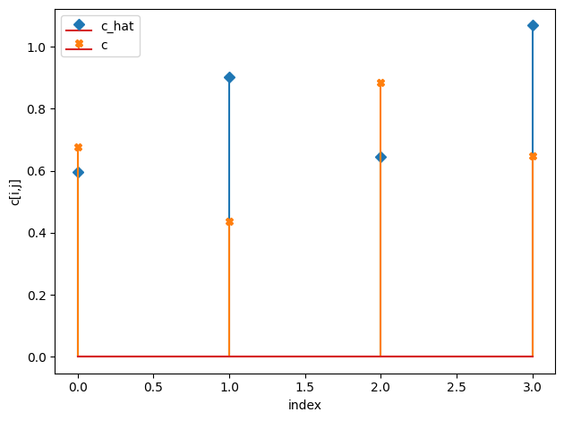
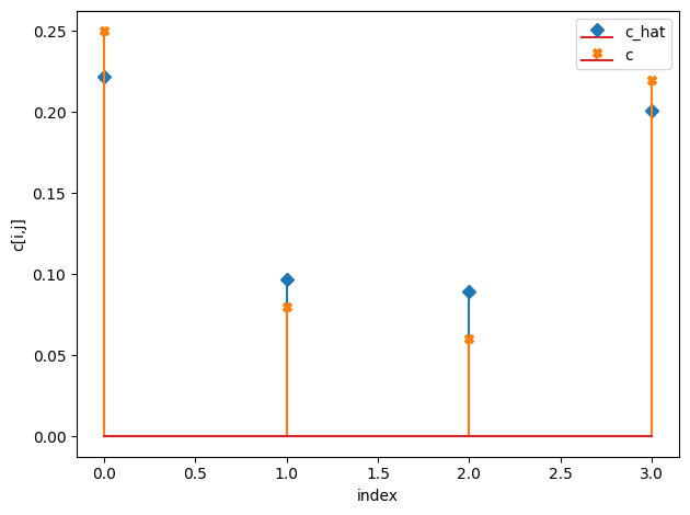
c_h = np.median(idata.posterior["c_hat"].values, axis=(0,1))
compare_params(c=(c, c_h))
predictor = sim_CRM()
predictor.set_parameters(num_species = num_species,
num_resources = num_resources,
tau = tau,
w = w,
c = c_h,
m = m,
r = r,
K = K)
#predictor.print_parameters()
observed_species, observed_resources = predictor.simulate(times, init_species)
observed_data = np.hstack((observed_species, observed_resources))
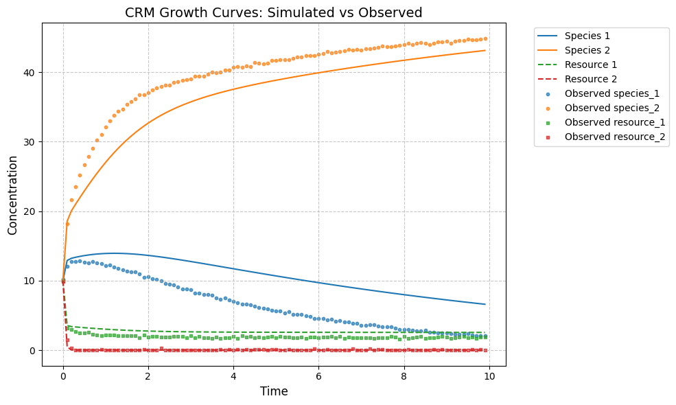
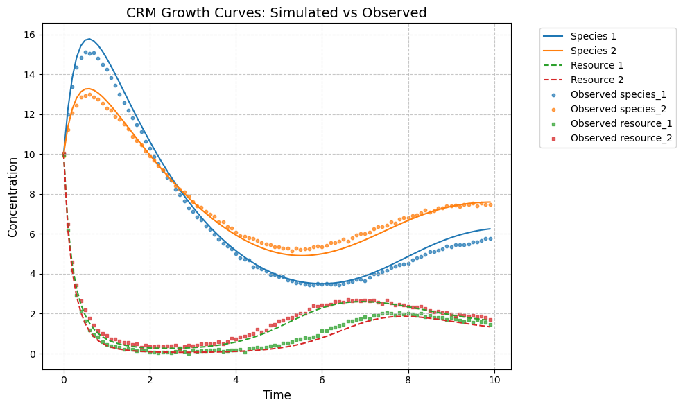
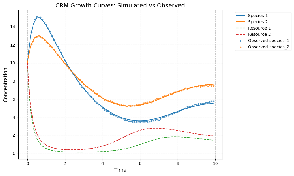
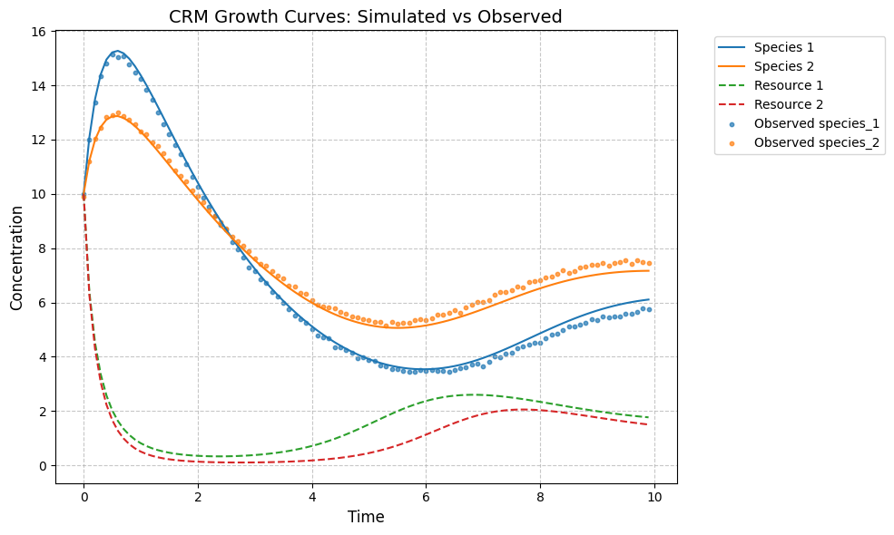
# plot predicted species and resouce dynamics against observed data
plot_CRM(observed_species, observed_resources, times, 'data-s2-r2.csv')
c_hat/c:
[[0.23 0.09]
 [0.08 0.21]]

 [[0.25 0.08]
 [0.06 0.22]]
[19]:
(<Figure size 1000x600 with 1 Axes>,
 <Axes: title={'center': 'CRM Growth Curves: Simulated vs Observed'}, xlabel='Time', ylabel='Concentration'>)
[20]:
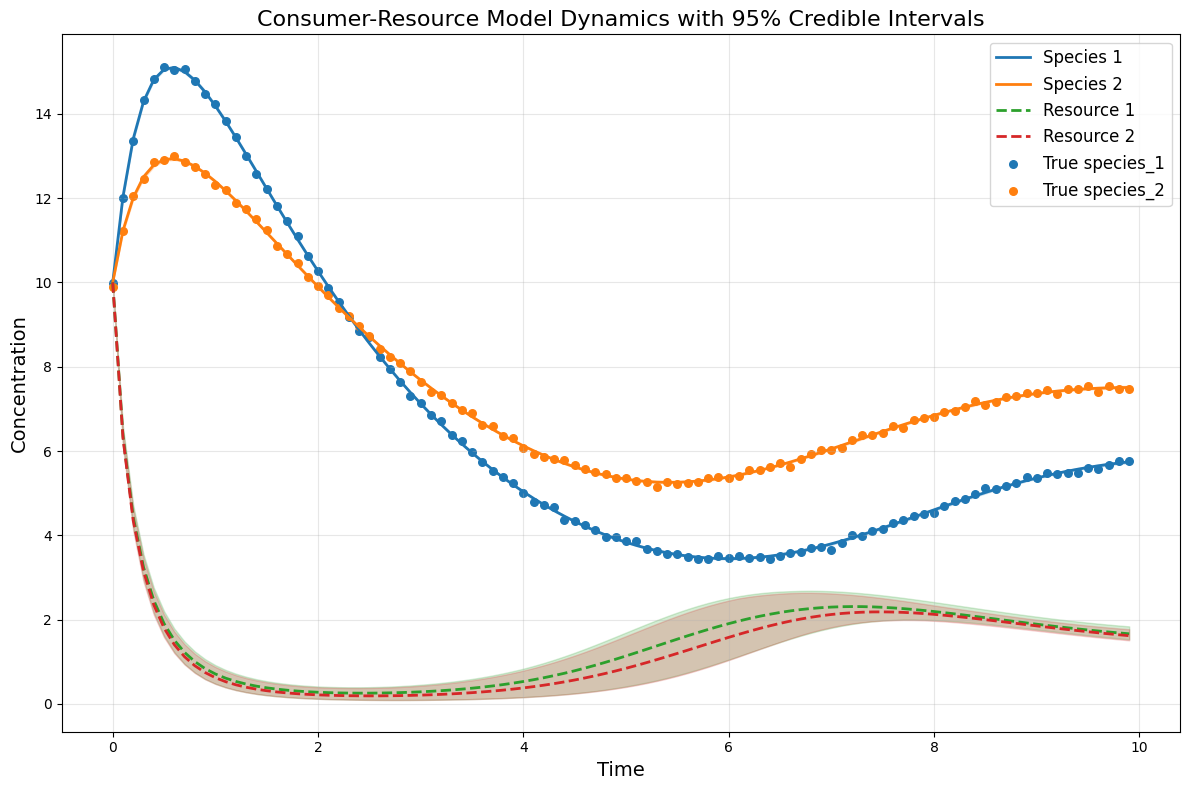
## Plot CRM with confidence intervals
# Get posterior samples for c_hat
c_posterior_samples = idata.posterior["c_hat"].values
lower_percentile = 2.5
upper_percentile = 97.5
n_samples = 50
random_indices = np.random.choice(c_posterior_samples.shape[1], size=n_samples, replace=False)
# Store simulation results
all_species_trajectories = []
all_resource_trajectories = []
# Run simulations with different posterior samples
for i in range(n_samples):
chain_idx = np.random.randint(0, c_posterior_samples.shape[0])
c_sample = c_posterior_samples[chain_idx, random_indices[i]]
sample_predictor = sim_CRM()
sample_predictor.set_parameters(num_species=num_species,
num_resources=num_resources,
tau=tau,
w=w,
c=c_sample,
m=m,
r=r,
K=K)
sample_species, sample_resources = sample_predictor.simulate(times, init_species)
# Store results
all_species_trajectories.append(sample_species)
all_resource_trajectories.append(sample_resources)
# Convert to numpy arrays
all_species_trajectories = np.array(all_species_trajectories)
all_resource_trajectories = np.array(all_resource_trajectories)
# Calculate percentiles across samples for each time point and species/resource
species_lower = np.percentile(all_species_trajectories, lower_percentile, axis=0)
species_median = np.median(all_species_trajectories, axis=0)
species_upper = np.percentile(all_species_trajectories, upper_percentile, axis=0)
resource_lower = np.percentile(all_resource_trajectories, lower_percentile, axis=0)
resource_median = np.median(all_resource_trajectories, axis=0)
resource_upper = np.percentile(all_resource_trajectories, upper_percentile, axis=0)
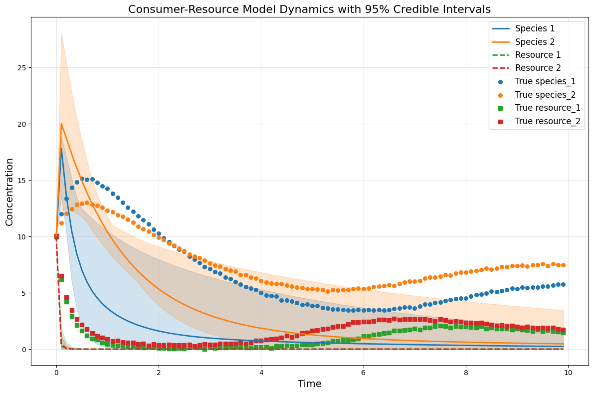
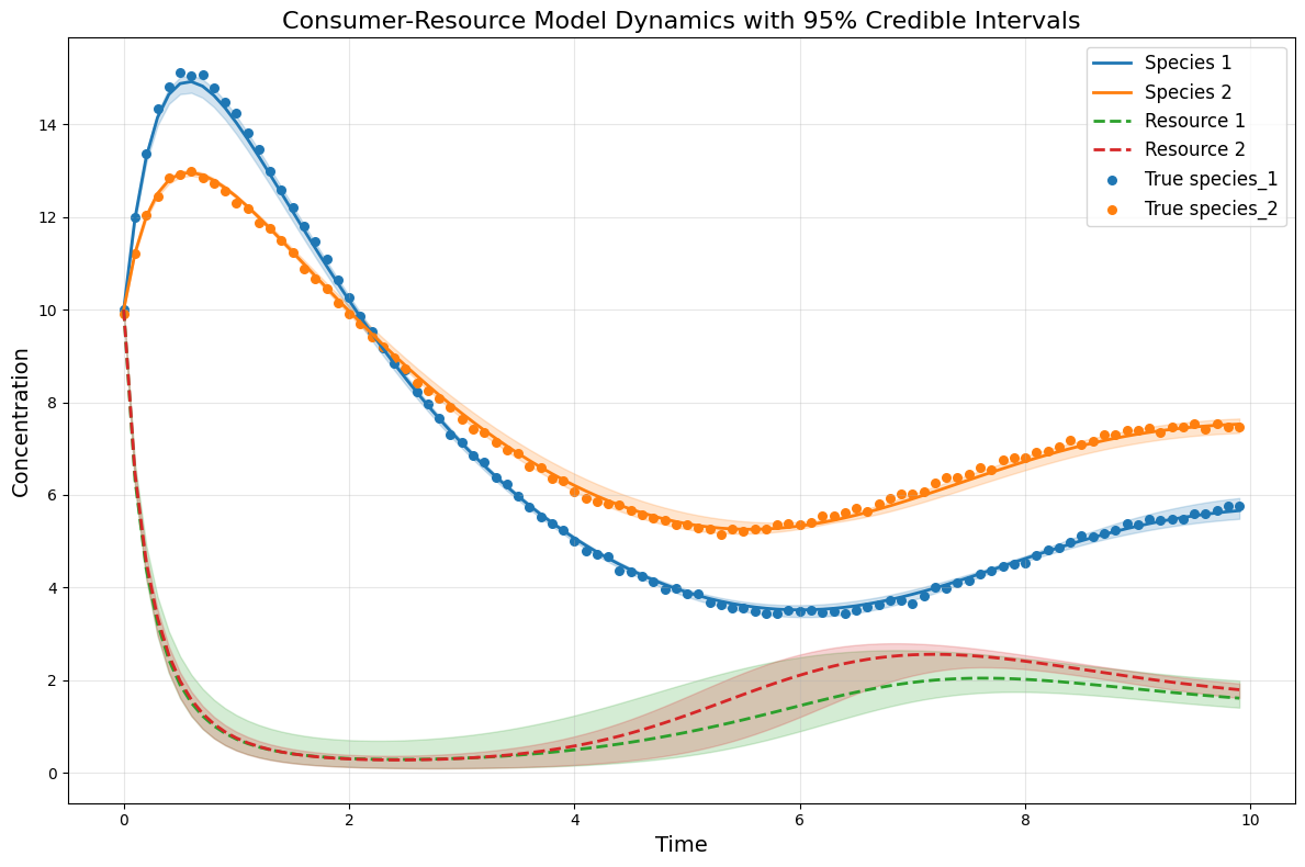
# plot the CRM with confidence intervals
plot_CRM_with_intervals(species_median, resource_median,
species_lower, species_upper,
resource_lower, resource_upper,
times, 'data-s2-r2.csv')
Infer all parameters
[3]:
num_species = 2
num_resources = 2
# fixed parameters
# tau = params["tau"]
# c = params["c"]
# m = params["m"]
# r = params["r"]
# w = params["w"]
# K = params["K"]
# Define prior for c (resource preference matrix)
prior_tau_mean = 0.7
prior_tau_sigma = 0.2
prior_w_mean = 0.55
prior_w_sigma = 0.2
prior_c_mean = 0.15
prior_c_sigma = 0.1
prior_m_mean = 0.25
prior_m_sigma = 0.1
prior_r_mean = 0.4
prior_r_sigma = 0.1
prior_K_mean = 5.5
prior_K_sigma = 0.5
# Sampling conditions
draws = 500
tune = 500
chains = 4
cores = 4
inference = inferCRMbayes()
inference.set_parameters(times=times, yobs=yobs, num_species=num_species, num_resources=num_resources,
prior_tau_mean=prior_tau_mean, prior_tau_sigma=prior_tau_sigma,
prior_w_mean=prior_w_mean, prior_w_sigma=prior_w_sigma,
prior_c_mean=prior_c_mean, prior_c_sigma=prior_c_sigma,
prior_m_mean=prior_m_mean, prior_m_sigma=prior_m_sigma,
prior_r_mean=prior_r_mean, prior_r_sigma=prior_r_sigma,
prior_K_mean=prior_K_mean, prior_K_sigma=prior_K_sigma,
draws=draws, tune=tune, chains=chains, cores=cores)
idata = inference.run_inference()
# To plot posterior distributions
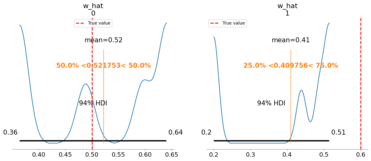
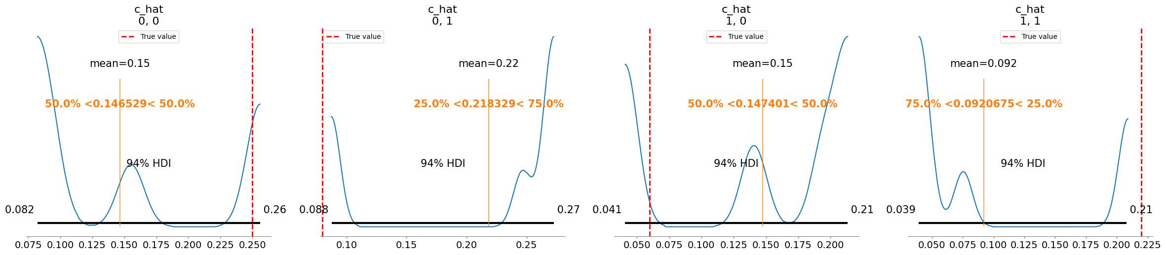
inference.plot_posterior(idata, true_params=params)
summary = az.summary(idata, var_names=["tau_hat", "w_hat","c_hat", "m_hat", "r_hat", "K_hat", "sigma"])
print(summary[["mean", "sd", "r_hat"]])
# Save posterior samples to file
az.to_netcdf(idata, 'model_posterior.nc')
times shape: (100,)
yobs shape: (100, 4)
Number of species: 2
Number of resources: 2
tau_hat is inferred
w_hat is inferred
c_hat is inferred
m_hat is inferred
r_hat is inferred
K_hat is inferred
=== RSME ===
RMSE with near-true parameters: 1.184889
Data scale: 4.327
Model scale: 4.895
First few predictions: [[10.         10.         10.         10.        ]
 [11.36026548 11.60057611  6.69560087  6.7189765 ]
 [12.32398306 12.73213984  4.81129297  4.95814782]]
First few observations: [[ 9.99394166  9.89957073  9.96255863 10.02837974]
 [12.00265551 11.21044161  6.20330201  6.50836833]
 [13.3618914  12.04261137  4.18667318  4.59287508]]
nsp_tensor: [2], nr_tensor: [2]
tau_hat: [0.47725705 0.7159908 ], w_hat: [0.46264173 0.49919912]
c_hat: [[0.15164175 0.03771675]
 [0.12005043 0.21566691]], m_hat: [0.11822559 0.26936813]
r_hat: [0.42827006 0.32282233], K_hat: [5.58117165 5.83735811]
theta: [2.         2.         0.47725705 0.7159908  0.46264173 0.49919912
 0.15164175 0.03771675 0.12005043 0.21566691 0.11822559 0.26936813
 0.42827006 0.32282233 5.58117165 5.83735811]
Initial conditions (y0): [10. 10. 10. 10.]
Auto-assigning NUTS sampler...
Initializing NUTS using jitter+adapt_diag...
Multiprocess sampling (4 chains in 4 jobs)
NUTS: [sigma, tau_hat, w_hat, c_hat_vals, m_hat, r_hat, K_hat]
/home/cclare/projects/CRM/MIMIC/MIMIC_env/lib/python3.10/site-packages/pymc/ode/ode.py:131: ODEintWarning: Illegal input detected (internal error). Run with full_output = 1 to get quantitative information.
  sol = scipy.integrate.odeint(
/home/cclare/projects/CRM/MIMIC/MIMIC_env/lib/python3.10/site-packages/pymc/ode/ode.py:131: ODEintWarning: Excess accuracy requested (tolerances too small). Run with full_output = 1 to get quantitative information.
  sol = scipy.integrate.odeint(
/home/cclare/projects/CRM/MIMIC/MIMIC_env/lib/python3.10/site-packages/pymc/ode/ode.py:131: ODEintWarning: Excess accuracy requested (tolerances too small). Run with full_output = 1 to get quantitative information.
  sol = scipy.integrate.odeint(
 lsoda--  warning..internal t (=r1) and h (=r2) are       such that in the machine, t + h = t on the next step
       (h = step size). solver will continue anyway      in above,  r1 =  0.0000000000000D+00   r2 =  0.0000000000000D+00
 intdy--  t (=r1) illegal            in above message,  r1 =  0.1000000000000D+00
      t not in interval tcur - hu (= r1) to tcur (=r2)
      in above,  r1 =  0.0000000000000D+00   r2 =  0.0000000000000D+00
 intdy--  t (=r1) illegal            in above message,  r1 =  0.2000000000000D+00
      t not in interval tcur - hu (= r1) to tcur (=r2)
      in above,  r1 =  0.0000000000000D+00   r2 =  0.0000000000000D+00
 lsoda--  trouble from intdy. itask = i1, tout = r1      in above message,  i1 =         1
      in above message,  r1 =  0.2000000000000D+00
 lsoda--  at t (=r1), too much accuracy requested         for precision of machine..  see tolsf (=r2)       in above,  r1 =  0.1000000000000D+00   r2 =                  NaN
 lsoda--  at t (=r1), too much accuracy requested         for precision of machine..  see tolsf (=r2)       in above,  r1 =  0.1000000000000D+00   r2 =                  NaN
 lsoda--  at t (=r1), too much accuracy requested         for precision of machine..  see tolsf (=r2)       in above,  r1 =  0.1000000000000D+00   r2 =                  NaN
/home/cclare/projects/CRM/MIMIC/MIMIC_env/lib/python3.10/site-packages/pymc/ode/ode.py:131: ODEintWarning: Excess work done on this call (perhaps wrong Dfun type). Run with full_output = 1 to get quantitative information.
  sol = scipy.integrate.odeint(
/home/cclare/projects/CRM/MIMIC/MIMIC_env/lib/python3.10/site-packages/pymc/ode/ode.py:131: ODEintWarning: Excess work done on this call (perhaps wrong Dfun type). Run with full_output = 1 to get quantitative information.
  sol = scipy.integrate.odeint(
/home/cclare/projects/CRM/MIMIC/MIMIC_env/lib/python3.10/site-packages/pymc/ode/ode.py:131: ODEintWarning: Illegal input detected (internal error). Run with full_output = 1 to get quantitative information.
  sol = scipy.integrate.odeint(
/home/cclare/projects/CRM/MIMIC/MIMIC_env/lib/python3.10/site-packages/pymc/ode/ode.py:131: ODEintWarning: Excess accuracy requested (tolerances too small). Run with full_output = 1 to get quantitative information.
  sol = scipy.integrate.odeint(
 intdy--  t (=r1) illegal            in above message,  r1 =  0.1000000000000D+00
      t not in interval tcur - hu (= r1) to tcur (=r2)
      in above,  r1 =  0.7165307645932D-23   r2 =  0.3940919205263D-22
 intdy--  t (=r1) illegal            in above message,  r1 =  0.2000000000000D+00
      t not in interval tcur - hu (= r1) to tcur (=r2)
      in above,  r1 =  0.7165307645932D-23   r2 =  0.3940919205263D-22
 lsoda--  trouble from intdy. itask = i1, tout = r1      in above message,  i1 =         1
      in above message,  r1 =  0.2000000000000D+00
 lsoda--  at t (=r1), too much accuracy requested         for precision of machine..  see tolsf (=r2)       in above,  r1 =  0.1000000000000D+00   r2 =                  NaN
/home/cclare/projects/CRM/MIMIC/MIMIC_env/lib/python3.10/site-packages/pymc/ode/ode.py:131: ODEintWarning: Excess work done on this call (perhaps wrong Dfun type). Run with full_output = 1 to get quantitative information.
  sol = scipy.integrate.odeint(
---------------------------------------------------------------------------
ValueError                                Traceback (most recent call last)
Cell In[3], line 53
     42 inference = inferCRMbayes()
     44 inference.set_parameters(times=times, yobs=yobs, num_species=num_species, num_resources=num_resources,
     45                             prior_tau_mean=prior_tau_mean, prior_tau_sigma=prior_tau_sigma,
     46                             prior_w_mean=prior_w_mean, prior_w_sigma=prior_w_sigma,
   (...)
     50                             prior_K_mean=prior_K_mean, prior_K_sigma=prior_K_sigma,
     51                          draws=draws, tune=tune, chains=chains, cores=cores)
---> 53 idata = inference.run_inference()
     55 # To plot posterior distributions
     56 inference.plot_posterior(idata, true_params=params)

File ~/projects/CRM/MIMIC/mimic/model_infer/infer_CRM_bayes.py:570, in inferCRMbayes.run_inference(self)
    567         print("Shape of crm_curves:", crm_curves.shape.eval())
    569     # Sample the posterior
--> 570     idata = pm.sample(draws=draws,tune=tune,chains=chains,cores=cores,progressbar=True)
    572 return idata

File ~/projects/CRM/MIMIC/MIMIC_env/lib/python3.10/site-packages/pymc/sampling/mcmc.py:877, in sample(draws, tune, chains, cores, random_seed, progressbar, progressbar_theme, step, var_names, nuts_sampler, initvals, init, jitter_max_retries, n_init, trace, discard_tuned_samples, compute_convergence_checks, keep_warning_stat, return_inferencedata, idata_kwargs, nuts_sampler_kwargs, callback, mp_ctx, blas_cores, model, **kwargs)
    873 t_sampling = time.time() - t_start
    875 # Packaging, validating and returning the result was extracted
    876 # into a function to make it easier to test and refactor.
--> 877 return _sample_return(
    878     run=run,
    879     traces=traces,
    880     tune=tune,
    881     t_sampling=t_sampling,
    882     discard_tuned_samples=discard_tuned_samples,
    883     compute_convergence_checks=compute_convergence_checks,
    884     return_inferencedata=return_inferencedata,
    885     keep_warning_stat=keep_warning_stat,
    886     idata_kwargs=idata_kwargs or {},
    887     model=model,
    888 )

File ~/projects/CRM/MIMIC/MIMIC_env/lib/python3.10/site-packages/pymc/sampling/mcmc.py:908, in _sample_return(run, traces, tune, t_sampling, discard_tuned_samples, compute_convergence_checks, return_inferencedata, keep_warning_stat, idata_kwargs, model)
    906 # Pick and slice chains to keep the maximum number of samples
    907 if discard_tuned_samples:
--> 908     traces, length = _choose_chains(traces, tune)
    909 else:
    910     traces, length = _choose_chains(traces, 0)

File ~/projects/CRM/MIMIC/MIMIC_env/lib/python3.10/site-packages/pymc/backends/base.py:593, in _choose_chains(traces, tune)
    591 lengths = [max(0, len(trace) - tune) for trace in traces]
    592 if not sum(lengths):
--> 593     raise ValueError("Not enough samples to build a trace.")
    595 idxs = np.argsort(lengths)
    596 l_sort = np.array(lengths)[idxs]

ValueError: Not enough samples to build a trace.
[20]:
summary = az.summary(idata, var_names=["tau_hat", "w_hat","c_hat", "m_hat", "r_hat", "K_hat", "sigma"])
print(summary[["mean", "sd", "r_hat"]])

# Save posterior samples to file
az.to_netcdf(idata, 'model_posterior.nc')

# To plot posterior distributions
inference.plot_posterior(idata, true_params=params)
mean sd r_hat
tau_hat[0] 0.578 0.100 4.43
tau_hat[1] 0.592 0.112 4.82
w_hat[0] 0.522 0.106 4.08
w_hat[1] 0.410 0.124 4.88
c_hat[0, 0] 0.147 0.069 3.33
c_hat[0, 1] 0.218 0.076 3.48
c_hat[1, 0] 0.147 0.067 3.20
c_hat[1, 1] 0.092 0.068 3.85
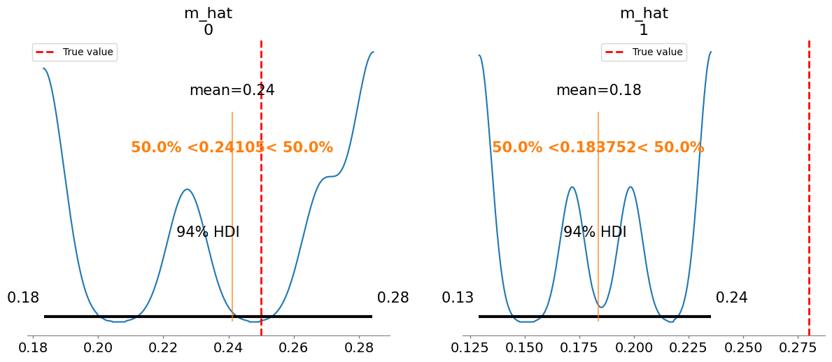
m_hat[0] 0.241 0.039 3.59
m_hat[1] 0.184 0.039 4.34
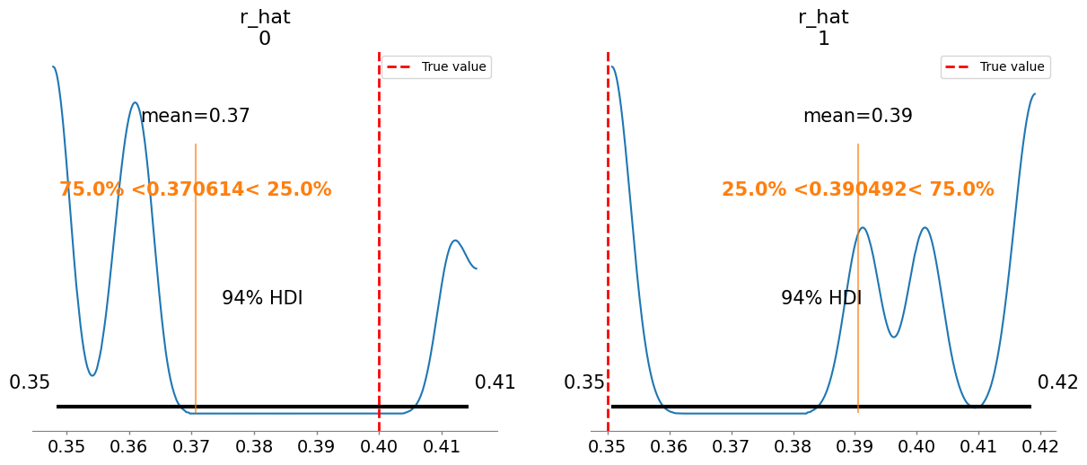
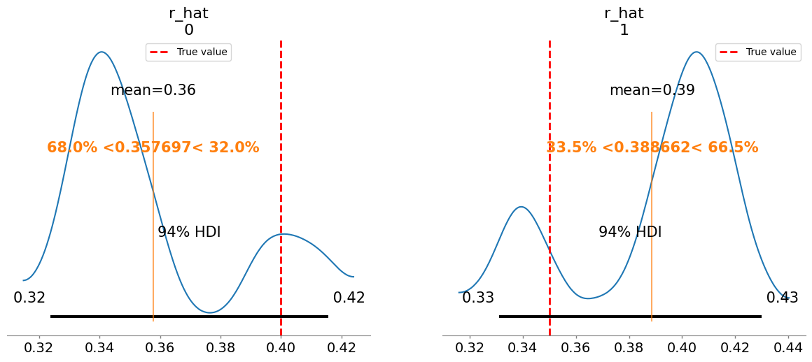
r_hat[0] 0.371 0.025 3.55
r_hat[1] 0.390 0.024 3.19
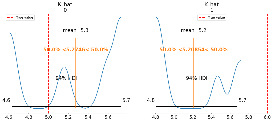
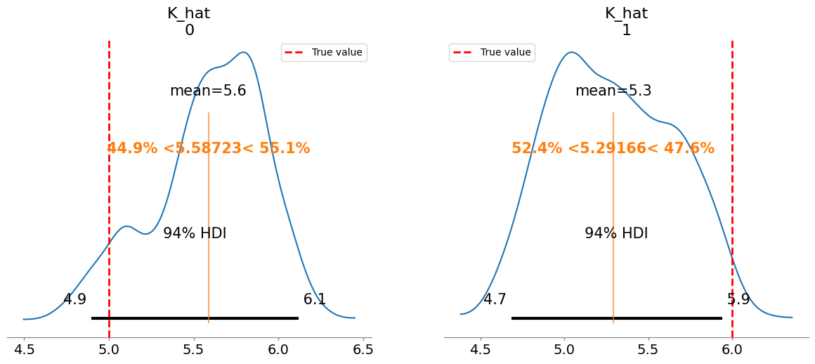
K_hat[0] 5.275 0.424 4.26
K_hat[1] 5.209 0.369 3.60
sigma[0] 0.073 0.039 4.87
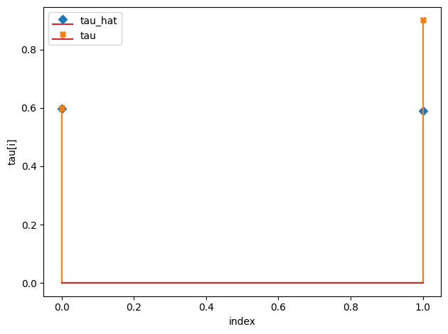
Plotting posterior for tau_hat
Added true value line for tau_hat: [0.6 0.9]
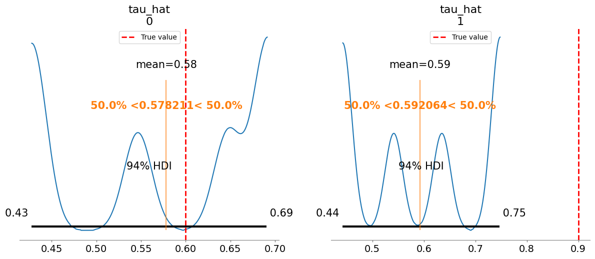
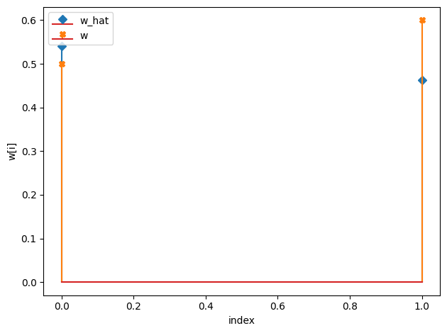
Plotting posterior for w_hat
Added true value line for w_hat: [0.5 0.6]
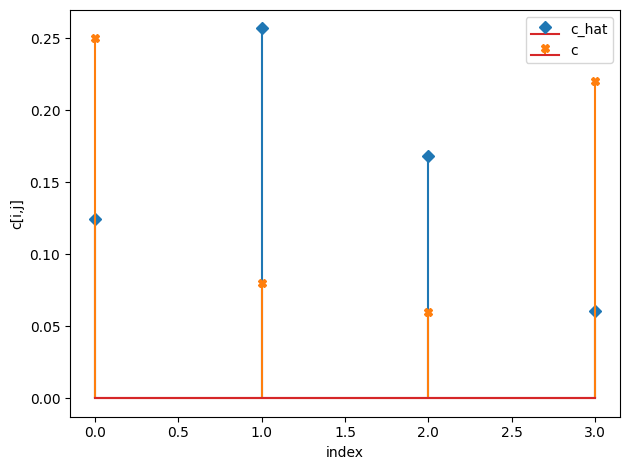
Plotting posterior for c_hat
Added true value line for c_hat: [[0.25 0.08]
 [0.06 0.22]]
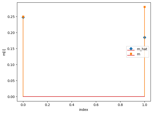
Plotting posterior for m_hat
Added true value line for m_hat: [0.25 0.28]
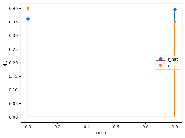
Plotting posterior for r_hat
Added true value line for r_hat: [0.4  0.35]
Plotting posterior for K_hat
Added true value line for K_hat: [5. 6.]
[11]:
# Plot the CRM
init_species = 10 * np.ones(num_species+num_resources)
# inferred parameters
tau_h = np.median(idata.posterior["tau_hat"].values, axis=(0,1))
w_h = np.median(idata.posterior["w_hat"].values, axis=(0,1))
c_h = np.median(idata.posterior["c_hat"].values, axis=(0,1))
m_h = np.median(idata.posterior["m_hat"].values, axis=(0,1))
r_h = np.median(idata.posterior["r_hat"].values, axis=(0,1))
K_h = np.median(idata.posterior["K_hat"].values, axis=(0,1))
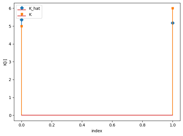
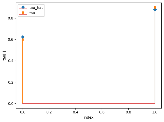
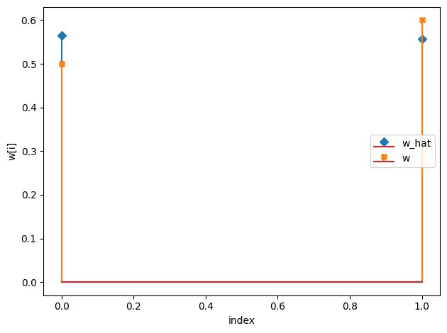
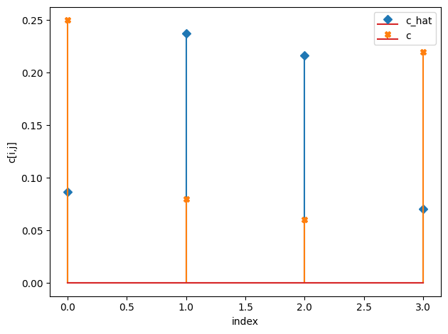
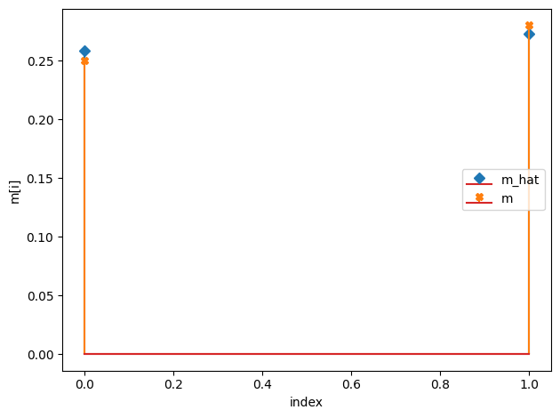
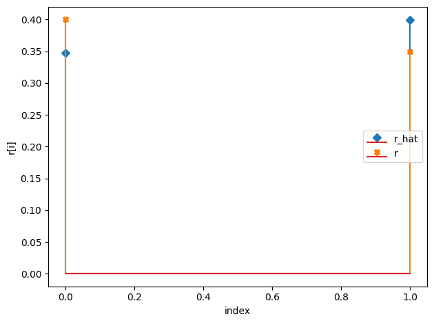
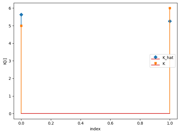
compare_params(tau=(tau, tau_h), w=(w, w_h), c=(c, c_h), m=(m, m_h), r=(r, r_h), K=(K, K_h))
predictor = sim_CRM()
predictor.set_parameters(num_species = num_species,
num_resources = num_resources,
tau = tau_h,
w = w_h,
c = c_h,
m = m_h,
r = r_h,
K = K_h)
#predictor.print_parameters()
observed_species, observed_resources = predictor.simulate(times, init_species)
observed_data = np.hstack((observed_species, observed_resources))
# plot predicted species and resouce dynamics against observed data
plot_CRM(observed_species, observed_resources, times, 'data-s2-r2.csv')
tau_hat/tau:
[0.6  0.59]

 [0.6 0.9]
w_hat/w:
[0.54 0.46]

 [0.5 0.6]
c_hat/c:
[[0.12 0.26]
 [0.17 0.06]]

 [[0.25 0.08]
 [0.06 0.22]]
m_hat/m:
[0.25 0.19]

 [0.25 0.28]
r_hat/r:
[0.36 0.4 ]

 [0.4  0.35]
K_hat/K:
[5.36 5.18]

 [5. 6.]
[11]:
(<Figure size 1000x600 with 1 Axes>,
 <Axes: title={'center': 'CRM Growth Curves: Simulated vs Observed'}, xlabel='Time', ylabel='Concentration'>)
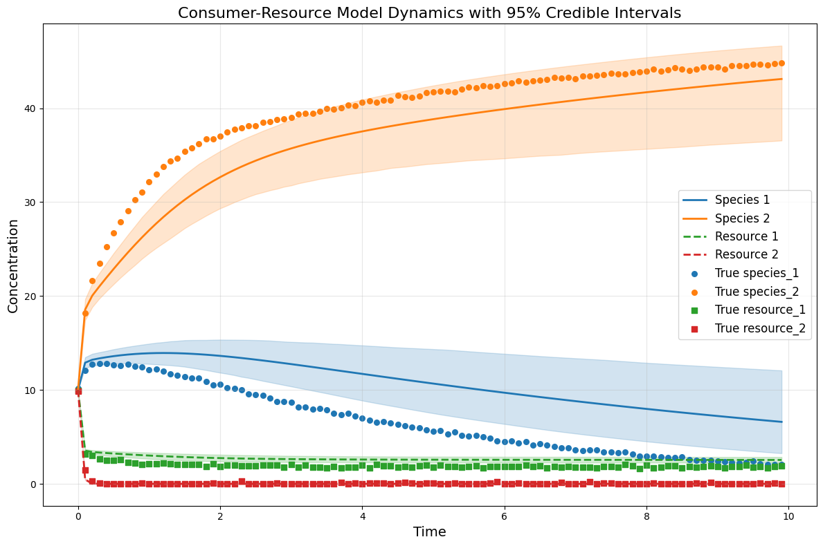
[23]:
## Plot CRM  with confidence intervals

# Get posterior samples for c_hat
tau_posterior_samples = idata.posterior["tau_hat"].values
w_posterior_samples = idata.posterior["w_hat"].values
c_posterior_samples = idata.posterior["c_hat"].values
m_posterior_samples = idata.posterior["m_hat"].values
r_posterior_samples = idata.posterior["r_hat"].values
K_posterior_samples = idata.posterior["K_hat"].values

lower_percentile = 2.5
upper_percentile = 97.5

n_samples = 10
random_indices = np.random.choice(c_posterior_samples.shape[1], size=n_samples, replace=False)

# Store simulation results
all_species_trajectories = []
all_resource_trajectories = []

# Run simulations with different posterior samples
for i in range(n_samples):
    chain_idx = np.random.randint(0, c_posterior_samples.shape[0])
    draw_idx = np.random.randint(0, c_posterior_samples.shape[1])

    tau_sample = tau_posterior_samples[chain_idx, draw_idx]
    w_sample = w_posterior_samples[chain_idx, draw_idx]
    c_sample = c_posterior_samples[chain_idx, draw_idx]
    m_sample = m_posterior_samples[chain_idx, draw_idx]
    r_sample = r_posterior_samples[chain_idx, draw_idx]
    K_sample = K_posterior_samples[chain_idx, draw_idx]

    sample_predictor = sim_CRM()
    sample_predictor.set_parameters(num_species=num_species,
                                   num_resources=num_resources,
                                   tau=tau_sample,
                                   w=w_sample,
                                   c=c_sample,
                                   m=m_sample,
                                   r=r_sample,
                                   K=K_sample)


    sample_species, sample_resources = sample_predictor.simulate(times, init_species)

    # Store results
    all_species_trajectories.append(sample_species)
    all_resource_trajectories.append(sample_resources)


# Convert to numpy arrays
all_species_trajectories = np.array(all_species_trajectories)
all_resource_trajectories = np.array(all_resource_trajectories)

# Calculate percentiles across samples for each time point and species/resource
species_lower = np.percentile(all_species_trajectories, lower_percentile, axis=0)
species_upper = np.percentile(all_species_trajectories, upper_percentile, axis=0)
resource_lower = np.percentile(all_resource_trajectories, lower_percentile, axis=0)
resource_upper = np.percentile(all_resource_trajectories, upper_percentile, axis=0)

observed_species_mean = np.mean(all_species_trajectories, axis=0)  # Predicted species means
observed_resources_mean = np.mean(all_resource_trajectories, axis=0)  # Predicted resources means

# plot the CRM with confidence intervals
plot_CRM_with_intervals(observed_species_mean, observed_resources_mean,
                       species_lower, species_upper,
                       resource_lower, resource_upper,
                       times, 'data-s2-r2.csv')
[ ]:
num_species = 2
num_resources = 2

# fixed parameters
# tau = params["tau"]
# c = params["c"]
# m = params["m"]
# r = params["r"]
# w = params["w"]
# K = params["K"]

# Define prior for c (resource preference matrix)


prior_tau_mean = 0.7
prior_tau_sigma = 0.2

prior_w_mean = 0.55
prior_w_sigma = 0.2

prior_c_mean = 0.15
prior_c_sigma = 0.1

prior_m_mean = 0.25
prior_m_sigma = 0.1

prior_r_mean = 0.4
prior_r_sigma = 0.1

prior_K_mean = 5.5
prior_K_sigma = 0.5


# Sampling conditions
draws = 500
tune = 500
chains = 4
cores = 4

inference = inferCRMbayes()

inference.set_parameters(times=times, yobs=yobs, num_species=num_species, num_resources=num_resources,
                            prior_tau_mean=prior_tau_mean, prior_tau_sigma=prior_tau_sigma,
                            prior_w_mean=prior_w_mean, prior_w_sigma=prior_w_sigma,
                            prior_c_mean=prior_c_mean, prior_c_sigma=prior_c_sigma,
                            prior_m_mean=prior_m_mean, prior_m_sigma=prior_m_sigma,
                            prior_r_mean=prior_r_mean, prior_r_sigma=prior_r_sigma,
                            prior_K_mean=prior_K_mean, prior_K_sigma=prior_K_sigma,
                         draws=draws, tune=tune, chains=chains, cores=cores)

idata = inference.run_inference()

# To plot posterior distributions
inference.plot_posterior(idata, true_params=params)


summary = az.summary(idata, var_names=["tau_hat", "w_hat","c_hat", "m_hat", "r_hat", "K_hat", "sigma"])
print(summary[["mean", "sd", "r_hat"]])

# Save posterior samples to file
az.to_netcdf(idata, 'model_posterior.nc')


# Plot the CRM

init_species = 10 * np.ones(num_species+num_resources)

# inferred parameters
tau_h = np.median(idata.posterior["tau_hat"].values, axis=(0,1))
w_h = np.median(idata.posterior["w_hat"].values, axis=(0,1))
c_h = np.median(idata.posterior["c_hat"].values, axis=(0,1))
m_h = np.median(idata.posterior["m_hat"].values, axis=(0,1))
r_h = np.median(idata.posterior["r_hat"].values, axis=(0,1))
K_h = np.median(idata.posterior["K_hat"].values, axis=(0,1))

compare_params(tau=(tau, tau_h), w=(w, w_h), c=(c, c_h), m=(m, m_h), r=(r, r_h), K=(K, K_h))

predictor = sim_CRM()

predictor.set_parameters(num_species = num_species,
                         num_resources = num_resources,
                         tau = tau_h,
                         w = w_h,
                         c = c_h,
                         m = m_h,
                         r = r_h,
                         K = K_h)

#predictor.print_parameters()

observed_species, observed_resources = predictor.simulate(times, init_species)
observed_data = np.hstack((observed_species, observed_resources))

# plot predicted species and resouce dynamics against observed data

plot_CRM(observed_species, observed_resources, times, 'data-s2-r2.csv')


## Plot CRM  with confidence intervals

# Get posterior samples for c_hat
tau_posterior_samples = idata.posterior["tau_hat"].values
w_posterior_samples = idata.posterior["w_hat"].values
c_posterior_samples = idata.posterior["c_hat"].values
m_posterior_samples = idata.posterior["m_hat"].values
r_posterior_samples = idata.posterior["r_hat"].values
K_posterior_samples = idata.posterior["K_hat"].values

lower_percentile = 2.5
upper_percentile = 97.5

n_samples = 10
random_indices = np.random.choice(c_posterior_samples.shape[1], size=n_samples, replace=False)

# Store simulation results
all_species_trajectories = []
all_resource_trajectories = []

# Run simulations with different posterior samples
for i in range(n_samples):
    chain_idx = np.random.randint(0, c_posterior_samples.shape[0])
    draw_idx = np.random.randint(0, c_posterior_samples.shape[1])

    tau_sample = tau_posterior_samples[chain_idx, draw_idx]
    w_sample = w_posterior_samples[chain_idx, draw_idx]
    c_sample = c_posterior_samples[chain_idx, draw_idx]
    m_sample = m_posterior_samples[chain_idx, draw_idx]
    r_sample = r_posterior_samples[chain_idx, draw_idx]
    K_sample = K_posterior_samples[chain_idx, draw_idx]

    sample_predictor = sim_CRM()
    sample_predictor.set_parameters(num_species=num_species,
                                   num_resources=num_resources,
                                   tau=tau_sample,
                                   w=w_sample,
                                   c=c_sample,
                                   m=m_sample,
                                   r=r_sample,
                                   K=K_sample)


    sample_species, sample_resources = sample_predictor.simulate(times, init_species)

    # Store results
    all_species_trajectories.append(sample_species)
    all_resource_trajectories.append(sample_resources)


# Convert to numpy arrays
all_species_trajectories = np.array(all_species_trajectories)
all_resource_trajectories = np.array(all_resource_trajectories)

# Calculate percentiles across samples for each time point and species/resource
species_lower = np.percentile(all_species_trajectories, lower_percentile, axis=0)
species_upper = np.percentile(all_species_trajectories, upper_percentile, axis=0)
resource_lower = np.percentile(all_resource_trajectories, lower_percentile, axis=0)
resource_upper = np.percentile(all_resource_trajectories, upper_percentile, axis=0)

observed_species_mean = np.mean(all_species_trajectories, axis=0)  # Predicted species means
observed_resources_mean = np.mean(all_resource_trajectories, axis=0)  # Predicted resources means

# plot the CRM with confidence intervals
plot_CRM_with_intervals(observed_species_mean, observed_resources_mean,
                       species_lower, species_upper,
                       resource_lower, resource_upper,
                       times, 'data-s2-r2.csv')
times shape: (100,)
yobs shape: (100, 4)
Number of species: 2
Number of resources: 2
tau_hat is inferred
w_hat is inferred
c_hat is inferred
m_hat is inferred
r_hat is inferred
K_hat is inferred
=== RSME ===
RMSE with near-true parameters: 2.420865
Data scale: 4.327
Model scale: 4.666
First few predictions: [[10.         10.         10.         10.        ]
 [11.07030377 10.62480967  6.73336742  7.57579737]
 [11.83386733 10.99784093  5.01400333  6.03867673]]
First few observations: [[ 9.99394166  9.89957073  9.96255863 10.02837974]
 [12.00265551 11.21044161  6.20330201  6.50836833]
 [13.3618914  12.04261137  4.18667318  4.59287508]]
nsp_tensor: [2], nr_tensor: [2]
tau_hat: [0.82251162 0.77451199], w_hat: [0.43984299 0.69477722]
c_hat: [[0.15388946 0.09513775]
 [0.06891893 0.09726492]], m_hat: [0.2903252  0.36499587]
r_hat: [0.40744778 0.47036901], K_hat: [4.92171108 6.38610421]
theta: [2.         2.         0.82251162 0.77451199 0.43984299 0.69477722
 0.15388946 0.09513775 0.06891893 0.09726492 0.2903252  0.36499587
 0.40744778 0.47036901 4.92171108 6.38610421]
Initial conditions (y0): [10. 10. 10. 10.]
Auto-assigning NUTS sampler...
Initializing NUTS using jitter+adapt_diag...
Multiprocess sampling (4 chains in 4 jobs)
NUTS: [sigma, tau_hat, w_hat, c_hat_vals, m_hat, r_hat, K_hat]
/home/cclare/projects/CRM/MIMIC/MIMIC_env/lib/python3.10/site-packages/pymc/ode/ode.py:131: ODEintWarning: Excess accuracy requested (tolerances too small). Run with full_output = 1 to get quantitative information.
  sol = scipy.integrate.odeint(
/home/cclare/projects/CRM/MIMIC/MIMIC_env/lib/python3.10/site-packages/pymc/ode/ode.py:131: ODEintWarning: Illegal input detected (internal error). Run with full_output = 1 to get quantitative information.
  sol = scipy.integrate.odeint(
/home/cclare/projects/CRM/MIMIC/MIMIC_env/lib/python3.10/site-packages/pymc/ode/ode.py:131: ODEintWarning: Excess accuracy requested (tolerances too small). Run with full_output = 1 to get quantitative information.
  sol = scipy.integrate.odeint(
 lsoda--  at t (=r1), too much accuracy requested         for precision of machine..  see tolsf (=r2)       in above,  r1 =  0.1000000000000D+00   r2 =                  NaN
 lsoda--  warning..internal t (=r1) and h (=r2) are       such that in the machine, t + h = t on the next step
       (h = step size). solver will continue anyway      in above,  r1 =  0.0000000000000D+00   r2 =  0.0000000000000D+00
 intdy--  t (=r1) illegal            in above message,  r1 =  0.1000000000000D+00
      t not in interval tcur - hu (= r1) to tcur (=r2)
      in above,  r1 =  0.0000000000000D+00   r2 =  0.0000000000000D+00
 intdy--  t (=r1) illegal            in above message,  r1 =  0.2000000000000D+00
      t not in interval tcur - hu (= r1) to tcur (=r2)
      in above,  r1 =  0.0000000000000D+00   r2 =  0.0000000000000D+00
 lsoda--  trouble from intdy. itask = i1, tout = r1      in above message,  i1 =         1
      in above message,  r1 =  0.2000000000000D+00
 lsoda--  at t (=r1), too much accuracy requested         for precision of machine..  see tolsf (=r2)       in above,  r1 =  0.1000000000000D+00   r2 =                  NaN
 lsoda--  at t (=r1), too much accuracy requested         for precision of machine..  see tolsf (=r2)       in above,  r1 =  0.1000000000000D+00   r2 =                  NaN
/home/cclare/projects/CRM/MIMIC/MIMIC_env/lib/python3.10/site-packages/pymc/ode/ode.py:131: ODEintWarning: Excess work done on this call (perhaps wrong Dfun type). Run with full_output = 1 to get quantitative information.
  sol = scipy.integrate.odeint(
/home/cclare/projects/CRM/MIMIC/MIMIC_env/lib/python3.10/site-packages/pymc/ode/ode.py:131: ODEintWarning: Excess accuracy requested (tolerances too small). Run with full_output = 1 to get quantitative information.
  sol = scipy.integrate.odeint(
lsoda-- at t (=r1), too much accuracy requested for precision of machine.. see tolsf (=r2) in above, r1 = 0.1000000000000D+00 r2 = NaN
[19]:
print("True parameters:")
print(f"w: {params['w']}")
print(f"r: {params['r']}")
print(f"K: {params['K']}")

print("Inferred parameters:")
print(f"w_hat: {np.median(idata.posterior['w_hat'].values, axis=(0,1))}")
print(f"r_hat: {np.median(idata.posterior['r_hat'].values, axis=(0,1))}")
print(f"K_hat: {np.median(idata.posterior['K_hat'].values, axis=(0,1))}")
True parameters:
w: [0.5 0.6]
r: [0.4  0.35]
K: [5. 6.]
Inferred parameters:
w_hat: [0.54140163 0.46366379]
r_hat: [0.36107019 0.39632932]
K_hat: [5.36404999 5.18260577]
Using only species data, infer resource concentration
[6]:
data = pd.read_csv("data-s2-infer-r2.csv")

times = data.iloc[:, 0].values
yobs = data.iloc[:, 1:3].values

print(params)
print(yobs)

num_species = 2
num_resources = 2

# fixed parameters
tau = params["tau"]
#c = params["c"]
m = params["m"]
r = params["r"]
w = params["w"]
K = params["K"]

# Define prior for c (resource preference matrix)

prior_c_mean = 0.15
prior_c_sigma = 0.1


# Sampling conditions
draws = 50
tune = 50
chains = 4
cores = 4

inference = inferCRMbayes()

inference.set_parameters(times=times, yobs=yobs, num_species=num_species, num_resources=num_resources,
                         tau=tau, w=w, K=K, r=r, m=m,
                         prior_c_mean=prior_c_mean, prior_c_sigma=prior_c_sigma,
                         draws=draws, tune=tune, chains=chains, cores=cores)

idata = inference.run_inference()

# To plot posterior distributions
inference.plot_posterior(idata, true_params=params)


summary = az.summary(idata, var_names=["c_hat", "sigma"])
print(summary[["mean", "sd", "r_hat"]])

# Save posterior samples to file
az.to_netcdf(idata, 'model_posterior.nc')
{'num_species': 2, 'num_resources': 2, 'tau': array([0.6, 0.9]), 'w': array([0.5, 0.6]), 'c': array([[0.25, 0.08],
       [0.06, 0.22]]), 'm': array([0.25, 0.28]), 'r': array([0.4 , 0.35]), 'K': array([5., 6.])}
[[ 9.99394166  9.89957073]
 [12.00265551 11.21044161]
 [13.3618914  12.04261137]
 [14.33843776 12.44382017]
 [14.82035602 12.84805998]
 [15.12285208 12.90998688]
 [15.04948901 12.9983141 ]
 [15.07148389 12.85380922]
 [14.78545571 12.7359763 ]
 [14.47296529 12.56154704]
 [14.24003097 12.30188608]
 [13.82041404 12.18159384]
 [13.45335285 11.88389378]
 [12.98808939 11.75275712]
 [12.57873255 11.49673126]
 [12.20735416 11.24393316]
 [11.80438777 10.87331634]
 [11.46742411 10.67239352]
 [11.10336494 10.46088776]
 [10.63444031 10.13934848]
 [10.27172776  9.9203375 ]
 [ 9.86151319  9.70606955]
 [ 9.53165117  9.40067621]
 [ 9.1815826   9.19638408]
 [ 8.84245445  8.9600867 ]
 [ 8.69522828  8.7249386 ]
 [ 8.22641928  8.42451177]
 [ 7.95315245  8.23888522]
 [ 7.64556214  8.09469538]
 [ 7.30251107  7.89419416]
 [ 7.1398518   7.62721272]
 [ 6.85123018  7.41291338]
 [ 6.70629555  7.34007131]
 [ 6.38546934  7.14126811]
 [ 6.22800166  6.97751262]
 [ 5.97480657  6.89790541]
 [ 5.73745883  6.6141611 ]
 [ 5.51952697  6.59421248]
 [ 5.38061968  6.35892698]
 [ 5.24917735  6.30260311]
 [ 5.01016103  6.08029617]
 [ 4.79772954  5.92304916]
 [ 4.71405836  5.85974041]
 [ 4.67990892  5.80693687]
 [ 4.35807892  5.7826572 ]
 [ 4.33990522  5.66292592]
 [ 4.25090495  5.56684272]
 [ 4.13623086  5.49679543]
 [ 3.95621657  5.44464471]
 [ 3.97235637  5.36594282]
 [ 3.8664521   5.3562975 ]
 [ 3.85544911  5.29030005]
 [ 3.68385719  5.27342975]
 [ 3.63510204  5.15063216]
 [ 3.55779398  5.27277504]
 [ 3.54712107  5.21969922]
 [ 3.47977964  5.25192898]
 [ 3.4462675   5.2620042 ]
 [ 3.44051009  5.35797886]
 [ 3.50719377  5.39271249]
 [ 3.47430715  5.35033518]
 [ 3.50518846  5.41624393]
 [ 3.47010094  5.55112086]
 [ 3.49229502  5.554409  ]
 [ 3.44383223  5.62932045]
 [ 3.4988675   5.72306934]
 [ 3.57880239  5.63221204]
 [ 3.6167633   5.80766636]
 [ 3.71168863  5.93058363]
 [ 3.72949937  6.02806988]
 [ 3.65128799  6.02390829]
 [ 3.82257323  6.08032998]
 [ 3.99900601  6.26862473]
 [ 3.98879135  6.37035053]
 [ 4.11237096  6.37427642]
 [ 4.15494146  6.43949156]
 [ 4.29749484  6.59261644]
 [ 4.37143486  6.53751897]
 [ 4.46078122  6.74603143]
 [ 4.49918578  6.79509641]
 [ 4.5258148   6.80371709]
 [ 4.68831847  6.91882804]
 [ 4.80630399  6.94063758]
 [ 4.85406473  7.03752194]
 [ 4.97773221  7.1912799 ]
 [ 5.11501462  7.0960825 ]
 [ 5.10130758  7.16912263]
 [ 5.17203069  7.29205137]
 [ 5.24748415  7.31050052]
 [ 5.38209153  7.38694469]
 [ 5.35507448  7.38598623]
 [ 5.46914818  7.44514603]
 [ 5.45730405  7.35186317]
 [ 5.46830484  7.47008933]
 [ 5.48321743  7.47365829]
 [ 5.59092956  7.54619268]
 [ 5.58488837  7.41121273]
 [ 5.6631945   7.54789487]
 [ 5.76736893  7.47600391]
 [ 5.76351915  7.46835014]]
times shape: (100,)
yobs shape: (100, 2)
Number of species: 2
Number of resources: 2
Only 50 samples per chain. Reliable r-hat and ESS diagnostics require longer chains for accurate estimate.
tau_hat is fixed
w_hat is fixed
c_hat is inferred
m_hat is fixed
r_hat is fixed
K_hat is fixed
=== CRITICAL: TESTING IF MODEL STRUCTURE IS CORRECT ===
MODEL FAILED: operands could not be broadcast together with shapes (100,4) (100,2)
nsp_tensor: [2], nr_tensor: [2]
tau_hat: [0.6 0.9], w_hat: [0.5 0.6]
c_hat: [[0.18037273 0.00144236]
 [0.18943669 0.1286244 ]], m_hat: [0.25 0.28]
r_hat: [0.4  0.35], K_hat: [5. 6.]
theta: [2.00000000e+00 2.00000000e+00 6.00000000e-01 9.00000000e-01
 5.00000000e-01 6.00000000e-01 1.80372728e-01 1.44235737e-03
 1.89436692e-01 1.28624405e-01 2.50000000e-01 2.80000000e-01
 4.00000000e-01 3.50000000e-01 5.00000000e+00 6.00000000e+00]
Initial conditions (y0): [10. 10. 10. 10.]
Auto-assigning NUTS sampler...
Initializing NUTS using jitter+adapt_diag...
Multiprocess sampling (4 chains in 4 jobs)
NUTS: [sigma, c_hat_vals]
/home/cclare/projects/CRM/MIMIC/MIMIC_env/lib/python3.10/site-packages/pymc/ode/ode.py:131: ODEintWarning: Illegal input detected (internal error). Run with full_output = 1 to get quantitative information.
  sol = scipy.integrate.odeint(
/home/cclare/projects/CRM/MIMIC/MIMIC_env/lib/python3.10/site-packages/pymc/ode/ode.py:131: ODEintWarning: Excess accuracy requested (tolerances too small). Run with full_output = 1 to get quantitative information.
  sol = scipy.integrate.odeint(
/home/cclare/projects/CRM/MIMIC/MIMIC_env/lib/python3.10/site-packages/pymc/ode/ode.py:131: ODEintWarning: Excess accuracy requested (tolerances too small). Run with full_output = 1 to get quantitative information.
  sol = scipy.integrate.odeint(
 lsoda--  warning..internal t (=r1) and h (=r2) are       such that in the machine, t + h = t on the next step
       (h = step size). solver will continue anyway      in above,  r1 =  0.0000000000000D+00   r2 =  0.0000000000000D+00
 intdy--  t (=r1) illegal            in above message,  r1 =  0.1000000000000D+00
      t not in interval tcur - hu (= r1) to tcur (=r2)
      in above,  r1 =  0.0000000000000D+00   r2 =  0.0000000000000D+00
 intdy--  t (=r1) illegal            in above message,  r1 =  0.2000000000000D+00
      t not in interval tcur - hu (= r1) to tcur (=r2)
      in above,  r1 =  0.0000000000000D+00   r2 =  0.0000000000000D+00
 lsoda--  trouble from intdy. itask = i1, tout = r1      in above message,  i1 =         1
      in above message,  r1 =  0.2000000000000D+00
 lsoda--  at t (=r1), too much accuracy requested         for precision of machine..  see tolsf (=r2)       in above,  r1 =  0.1000000000000D+00   r2 =                  NaN
 lsoda--  at t (=r1), too much accuracy requested         for precision of machine..  see tolsf (=r2)       in above,  r1 =  0.1000000000000D+00   r2 =                  NaN
 lsoda--  at t (=r1), too much accuracy requested         for precision of machine..  see tolsf (=r2)       in above,  r1 =  0.1000000000000D+00   r2 =                  NaN
/home/cclare/projects/CRM/MIMIC/MIMIC_env/lib/python3.10/site-packages/pymc/ode/ode.py:131: ODEintWarning: Excess work done on this call (perhaps wrong Dfun type). Run with full_output = 1 to get quantitative information.
  sol = scipy.integrate.odeint(
/home/cclare/projects/CRM/MIMIC/MIMIC_env/lib/python3.10/site-packages/pymc/ode/ode.py:131: ODEintWarning: Excess work done on this call (perhaps wrong Dfun type). Run with full_output = 1 to get quantitative information.
  sol = scipy.integrate.odeint(
/home/cclare/projects/CRM/MIMIC/MIMIC_env/lib/python3.10/site-packages/pymc/ode/ode.py:131: ODEintWarning: Excess accuracy requested (tolerances too small). Run with full_output = 1 to get quantitative information.
  sol = scipy.integrate.odeint(
/home/cclare/projects/CRM/MIMIC/MIMIC_env/lib/python3.10/site-packages/pymc/ode/ode.py:131: ODEintWarning: Excess accuracy requested (tolerances too small). Run with full_output = 1 to get quantitative information.
  sol = scipy.integrate.odeint(
 lsoda--  at t (=r1), too much accuracy requested         for precision of machine..  see tolsf (=r2)       in above,  r1 =  0.1000000000000D+00   r2 =                  NaN
 lsoda--  at t (=r1), too much accuracy requested         for precision of machine..  see tolsf (=r2)       in above,  r1 =  0.1000000000000D+00   r2 =                  NaN
Sampling 4 chains for 50 tune and 50 draw iterations (200 + 200 draws total) took 115 seconds.
There were 44 divergences after tuning. Increase `target_accept` or reparameterize.
The number of samples is too small to check convergence reliably.
Parameter tau_hat not found in posterior samples, skipping plot.
Parameter w_hat not found in posterior samples, skipping plot.
Plotting posterior for c_hat
Added true value line for c_hat: [[0.25 0.08]
 [0.06 0.22]]
Parameter m_hat not found in posterior samples, skipping plot.
Parameter r_hat not found in posterior samples, skipping plot.
Parameter K_hat not found in posterior samples, skipping plot.
              mean     sd  r_hat
c_hat[0, 0]  0.185  0.070   3.03
c_hat[0, 1]  0.126  0.054   2.99
c_hat[1, 0]  0.107  0.035   3.04
c_hat[1, 1]  0.185  0.031   3.10
sigma[0]     0.183  0.036   3.52
[6]:
'model_posterior.nc'
[7]:
# Plot the trace of the posterior samples
az.plot_trace(idata, var_names=["c_hat", "sigma"])
[7]:
array([[<Axes: title={'center': 'c_hat'}>,
        <Axes: title={'center': 'c_hat'}>],
       [<Axes: title={'center': 'sigma'}>,
        <Axes: title={'center': 'sigma'}>]], dtype=object)
[ ]:
[8]:
# Plot the CRM

init_species = 10 * np.ones(num_species+num_resources)

# inferred parameters
c_h = np.median(idata.posterior["c_hat"].values, axis=(0,1))

compare_params(c=(c, c_h))

predictor = sim_CRM()

predictor.set_parameters(num_species = num_species,
                         num_resources = num_resources,
                         tau = tau,
                         w = w,
                         c = c_h,
                         m = m,
                         r = r,
                         K = K)

#predictor.print_parameters()

observed_species, observed_resources = predictor.simulate(times, init_species)
observed_data = np.hstack((observed_species, observed_resources))

# plot predicted species and resouce dynamics against observed data

plot_CRM(observed_species, observed_resources, times, 'data-s2-infer-r2.csv')
c_hat/c:
[[0.22 0.1 ]
 [0.09 0.2 ]]

 [[0.25 0.08]
 [0.06 0.22]]
[8]:
(<Figure size 1000x600 with 1 Axes>,
 <Axes: title={'center': 'CRM Growth Curves: Simulated vs Observed'}, xlabel='Time', ylabel='Concentration'>)
[9]:
## Plot CRM  with confidence intervals

# Get posterior samples for c_hat
c_posterior_samples = idata.posterior["c_hat"].values

lower_percentile = 2.5
upper_percentile = 97.5

n_samples = 50
random_indices = np.random.choice(c_posterior_samples.shape[1], size=n_samples, replace=False)

# Store simulation results
all_species_trajectories = []
all_resource_trajectories = []

# Run simulations with different posterior samples
for i in range(n_samples):
    chain_idx = np.random.randint(0, c_posterior_samples.shape[0])
    draw_idx = np.random.randint(0, c_posterior_samples.shape[1])

    c_sample = c_posterior_samples[chain_idx, draw_idx]

    sample_predictor = sim_CRM()
    sample_predictor.set_parameters(num_species=num_species,
                                   num_resources=num_resources,
                                   tau=tau,
                                   w=w,
                                   c=c_sample,
                                   m=m,
                                   r=r,
                                   K=K)


    sample_species, sample_resources = sample_predictor.simulate(times, init_species)

    # Store results
    all_species_trajectories.append(sample_species)
    all_resource_trajectories.append(sample_resources)


# Convert to numpy arrays
all_species_trajectories = np.array(all_species_trajectories)
all_resource_trajectories = np.array(all_resource_trajectories)

# Calculate percentiles across samples for each time point and species/resource
species_lower = np.percentile(all_species_trajectories, lower_percentile, axis=0)
species_upper = np.percentile(all_species_trajectories, upper_percentile, axis=0)
resource_lower = np.percentile(all_resource_trajectories, lower_percentile, axis=0)
resource_upper = np.percentile(all_resource_trajectories, upper_percentile, axis=0)

observed_species_mean = np.mean(all_species_trajectories, axis=0)  # Predicted species means
observed_resources_mean = np.mean(all_resource_trajectories, axis=0)  # Predicted resources means

# plot the CRM with confidence intervals
plot_CRM_with_intervals(observed_species_mean, observed_resources_mean,
                       species_lower, species_upper,
                       resource_lower, resource_upper,
                       times, 'data-s2-infer-r2.csv')
Infer all parameters when only given species data
[15]:
data = pd.read_csv("data-s2-infer-r2.csv")

times = data.iloc[:, 0].values
yobs = data.iloc[:, 1:3].values


num_species = 2
num_resources = 2


prior_tau_mean = 0.7
prior_tau_sigma = 0.2

prior_w_mean = 0.55
prior_w_sigma = 0.2

prior_c_mean = 0.15
prior_c_sigma = 0.1

prior_m_mean = 0.25
prior_m_sigma = 0.1

prior_r_mean = 0.4
prior_r_sigma = 0.1

prior_K_mean = 5.5
prior_K_sigma = 0.5


# Sampling conditions
draws = 200
tune = 200
chains = 4
cores = 4

inference = inferCRMbayes()

inference.set_parameters(times=times, yobs=yobs, num_species=num_species, num_resources=num_resources,
                            prior_tau_mean=prior_tau_mean, prior_tau_sigma=prior_tau_sigma,
                            prior_w_mean=prior_w_mean, prior_w_sigma=prior_w_sigma,
                            prior_c_mean=prior_c_mean, prior_c_sigma=prior_c_sigma,
                            prior_m_mean=prior_m_mean, prior_m_sigma=prior_m_sigma,
                            prior_r_mean=prior_r_mean, prior_r_sigma=prior_r_sigma,
                            prior_K_mean=prior_K_mean, prior_K_sigma=prior_K_sigma,
                         draws=draws, tune=tune, chains=chains, cores=cores)

idata = inference.run_inference()

# To plot posterior distributions
inference.plot_posterior(idata, true_params=params)


summary = az.summary(idata, var_names=["tau_hat", "w_hat","c_hat", "m_hat", "r_hat", "K_hat", "sigma"])
print(summary[["mean", "sd", "r_hat"]])

# Save posterior samples to file
az.to_netcdf(idata, 'model_posterior.nc')
times shape: (100,)
yobs shape: (100, 2)
Number of species: 2
Number of resources: 2
tau_hat is inferred
w_hat is inferred
c_hat is inferred
m_hat is inferred
r_hat is inferred
K_hat is inferred
=== CRITICAL: TESTING IF MODEL STRUCTURE IS CORRECT ===
MODEL FAILED: operands could not be broadcast together with shapes (100,4) (100,2)
nsp_tensor: [2], nr_tensor: [2]
tau_hat: [0.83790865 0.61771527], w_hat: [0.85862258 0.51106388]
c_hat: [[0.04790821 0.26154852]
 [0.15444959 0.32360037]], m_hat: [0.25944519 0.36373094]
r_hat: [0.40526451 0.34769188], K_hat: [5.30127861 5.81092244]
theta: [2.         2.         0.83790865 0.61771527 0.85862258 0.51106388
 0.04790821 0.26154852 0.15444959 0.32360037 0.25944519 0.36373094
 0.40526451 0.34769188 5.30127861 5.81092244]
Initial conditions (y0): [10. 10. 10. 10.]
Auto-assigning NUTS sampler...
Initializing NUTS using jitter+adapt_diag...
Multiprocess sampling (4 chains in 4 jobs)
NUTS: [sigma, tau_hat, w_hat, c_hat_vals, m_hat, r_hat, K_hat]
/home/cclare/projects/CRM/MIMIC/MIMIC_env/lib/python3.10/site-packages/pymc/ode/ode.py:131: ODEintWarning: Excess accuracy requested (tolerances too small). Run with full_output = 1 to get quantitative information.
  sol = scipy.integrate.odeint(
/home/cclare/projects/CRM/MIMIC/MIMIC_env/lib/python3.10/site-packages/pymc/ode/ode.py:131: ODEintWarning: Excess accuracy requested (tolerances too small). Run with full_output = 1 to get quantitative information.
  sol = scipy.integrate.odeint(
 lsoda--  at t (=r1), too much accuracy requested         for precision of machine..  see tolsf (=r2)       in above,  r1 =  0.1000000000000D+00   r2 =                  NaN
 lsoda--  at t (=r1), too much accuracy requested         for precision of machine..  see tolsf (=r2)       in above,  r1 =  0.1000000000000D+00   r2 =                  NaN
 lsoda--  at t (=r1), too much accuracy requested         for precision of machine..  see tolsf (=r2)       in above,  r1 =  0.1000000000000D+00   r2 =                  NaN
 lsoda--  at t (=r1), too much accuracy requested         for precision of machine..  see tolsf (=r2)       in above,  r1 =  0.1000000000000D+00   r2 =                  NaN
/home/cclare/projects/CRM/MIMIC/MIMIC_env/lib/python3.10/site-packages/pymc/ode/ode.py:131: ODEintWarning: Excess accuracy requested (tolerances too small). Run with full_output = 1 to get quantitative information.
  sol = scipy.integrate.odeint(
/home/cclare/projects/CRM/MIMIC/MIMIC_env/lib/python3.10/site-packages/pymc/ode/ode.py:131: ODEintWarning: Excess accuracy requested (tolerances too small). Run with full_output = 1 to get quantitative information.
  sol = scipy.integrate.odeint(
 lsoda--  at t (=r1), too much accuracy requested         for precision of machine..  see tolsf (=r2)       in above,  r1 =  0.1000000000000D+00   r2 =                  NaN
 lsoda--  at t (=r1), too much accuracy requested         for precision of machine..  see tolsf (=r2)       in above,  r1 =  0.1000000000000D+00   r2 =                  NaN
Sampling 4 chains for 200 tune and 200 draw iterations (800 + 800 draws total) took 15924 seconds.
Chain 0 reached the maximum tree depth. Increase `max_treedepth`, increase `target_accept` or reparameterize.
Chain 1 reached the maximum tree depth. Increase `max_treedepth`, increase `target_accept` or reparameterize.
Chain 2 reached the maximum tree depth. Increase `max_treedepth`, increase `target_accept` or reparameterize.
Chain 3 reached the maximum tree depth. Increase `max_treedepth`, increase `target_accept` or reparameterize.
The rhat statistic is larger than 1.01 for some parameters. This indicates problems during sampling. See https://arxiv.org/abs/1903.08008 for details
The effective sample size per chain is smaller than 100 for some parameters.  A higher number is needed for reliable rhat and ess computation. See https://arxiv.org/abs/1903.08008 for details
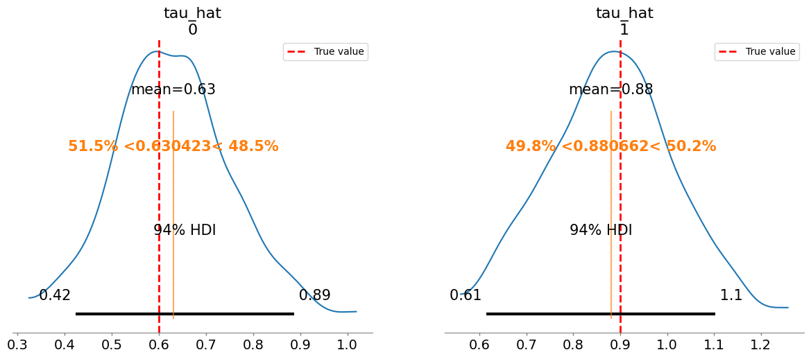
Plotting posterior for tau_hat
Added true value line for tau_hat: [0.6 0.9]
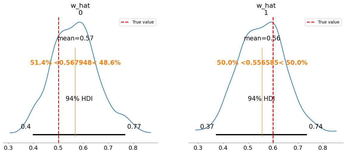
Plotting posterior for w_hat
Added true value line for w_hat: [0.5 0.6]
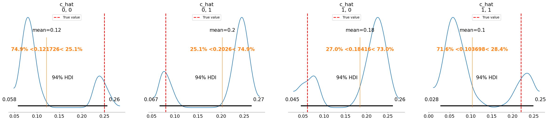
Plotting posterior for c_hat
Added true value line for c_hat: [[0.25 0.08]
 [0.06 0.22]]
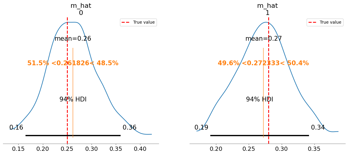
Plotting posterior for m_hat
Added true value line for m_hat: [0.25 0.28]
Plotting posterior for r_hat
Added true value line for r_hat: [0.4  0.35]
Plotting posterior for K_hat
Added true value line for K_hat: [5. 6.]
              mean     sd  r_hat
tau_hat[0]   0.630  0.120   1.03
tau_hat[1]   0.881  0.131   1.01
w_hat[0]     0.568  0.098   1.03
w_hat[1]     0.557  0.097   1.02
c_hat[0, 0]  0.122  0.071   1.57
c_hat[0, 1]  0.203  0.072   1.57
c_hat[1, 0]  0.184  0.072   1.57
c_hat[1, 1]  0.104  0.075   1.56
m_hat[0]     0.262  0.050   1.03
m_hat[1]     0.272  0.040   1.01
r_hat[0]     0.358  0.029   1.56
r_hat[1]     0.389  0.031   1.54
K_hat[0]     5.587  0.338   1.36
K_hat[1]     5.292  0.369   1.37
sigma[0]     0.049  0.003   1.01
[15]:
'model_posterior.nc'
[16]:
# Plot the CRM

init_species = 10 * np.ones(num_species+num_resources)

# inferred parameters
tau_h = np.median(idata.posterior["tau_hat"].values, axis=(0,1))
w_h = np.median(idata.posterior["w_hat"].values, axis=(0,1))
c_h = np.median(idata.posterior["c_hat"].values, axis=(0,1))
m_h = np.median(idata.posterior["m_hat"].values, axis=(0,1))
r_h = np.median(idata.posterior["r_hat"].values, axis=(0,1))
K_h = np.median(idata.posterior["K_hat"].values, axis=(0,1))

compare_params(tau=(tau, tau_h), w=(w, w_h), c=(c, c_h), m=(m, m_h), r=(r, r_h), K=(K, K_h))

predictor = sim_CRM()

predictor.set_parameters(num_species = num_species,
                         num_resources = num_resources,
                         tau = tau_h,
                         w = w_h,
                         c = c_h,
                         m = m_h,
                         r = r_h,
                         K = K_h)

#predictor.print_parameters()

observed_species, observed_resources = predictor.simulate(times, init_species)
observed_data = np.hstack((observed_species, observed_resources))

# plot predicted species and resouce dynamics against observed data

plot_CRM(observed_species, observed_resources, times, 'data-s2-infer-r2.csv')
tau_hat/tau:
[0.62 0.88]

 [0.6 0.9]
w_hat/w:
[0.56 0.56]

 [0.5 0.6]
c_hat/c:
[[0.09 0.24]
 [0.22 0.07]]

 [[0.25 0.08]
 [0.06 0.22]]
m_hat/m:
[0.26 0.27]

 [0.25 0.28]
r_hat/r:
[0.35 0.4 ]

 [0.4  0.35]
K_hat/K:
[5.63 5.27]

 [5. 6.]
[16]:
(<Figure size 1000x600 with 1 Axes>,
 <Axes: title={'center': 'CRM Growth Curves: Simulated vs Observed'}, xlabel='Time', ylabel='Concentration'>)
[17]:
## Plot CRM  with confidence intervals

# Get posterior samples for c_hat
tau_posterior_samples = idata.posterior["tau_hat"].values
w_posterior_samples = idata.posterior["w_hat"].values
c_posterior_samples = idata.posterior["c_hat"].values
m_posterior_samples = idata.posterior["m_hat"].values
r_posterior_samples = idata.posterior["r_hat"].values
K_posterior_samples = idata.posterior["K_hat"].values

lower_percentile = 2.5
upper_percentile = 97.5

n_samples = 50
random_indices = np.random.choice(c_posterior_samples.shape[1], size=n_samples, replace=False)

# Store simulation results
all_species_trajectories = []
all_resource_trajectories = []

# Run simulations with different posterior samples
for i in range(n_samples):
    chain_idx = np.random.randint(0, c_posterior_samples.shape[0])
    draw_idx = np.random.randint(0, c_posterior_samples.shape[1])

    tau_sample = tau_posterior_samples[chain_idx, draw_idx]
    w_sample = w_posterior_samples[chain_idx, draw_idx]
    c_sample = c_posterior_samples[chain_idx, draw_idx]
    m_sample = m_posterior_samples[chain_idx, draw_idx]
    r_sample = r_posterior_samples[chain_idx, draw_idx]
    K_sample = K_posterior_samples[chain_idx, draw_idx]

    sample_predictor = sim_CRM()
    sample_predictor.set_parameters(num_species=num_species,
                                   num_resources=num_resources,
                                   tau=tau_sample,
                                   w=w_sample,
                                   c=c_sample,
                                   m=m_sample,
                                   r=r_sample,
                                   K=K_sample)


    sample_species, sample_resources = sample_predictor.simulate(times, init_species)

    # Store results
    all_species_trajectories.append(sample_species)
    all_resource_trajectories.append(sample_resources)


# Convert to numpy arrays
all_species_trajectories = np.array(all_species_trajectories)
all_resource_trajectories = np.array(all_resource_trajectories)

# Calculate percentiles across samples for each time point and species/resource
species_lower = np.percentile(all_species_trajectories, lower_percentile, axis=0)
species_upper = np.percentile(all_species_trajectories, upper_percentile, axis=0)
resource_lower = np.percentile(all_resource_trajectories, lower_percentile, axis=0)
resource_upper = np.percentile(all_resource_trajectories, upper_percentile, axis=0)

observed_species_mean = np.mean(all_species_trajectories, axis=0)  # Predicted species means
observed_resources_mean = np.mean(all_resource_trajectories, axis=0)  # Predicted resources means

# plot the CRM with confidence intervals
plot_CRM_with_intervals(observed_species_mean, observed_resources_mean,
                       species_lower, species_upper,
                       resource_lower, resource_upper,
                       times, 'data-s2-infer-r2.csv')
[ ]: